Final Project

Goals and Background
Throughout the semester I have learned many GIS techniques within lecture and by completing tutorials and labs to the best of my ability.  The information I have retained has been crucial in the completion of my final project.  This includes knowledge I have gained about setting up file geodatabases, queries, making new feature classes, coordinate systems, geoprocessing tools, and python scripting.  The goal of this project was to evaluate the GIS skills I have learned throughout this course to solve a spatial question of my choosing.  The question that I chose to assess went as follows: "Is there a potential correlation between the concentrations of diesel particulate matter (PM) in proximity to main interstates within the Central Valley and is this relationship connected to the rate of asthma emergency department visits among California residents?"  Additional objectives include using a minimum of three different spatial layers and four tools and further create maps and a data flow model that display the analysis of my spatial question.

Methods
To begin my protect, I searched for data that was relevant to my data; ArcGIS online provided the most relevant and useful data that I could find.  I added the layers I needed from both the US geodatabase used in the Price tutorials and from ArcGIS online.  I then set the projection of each layer to the UTM Zone 11N because it was the best fit for the Central Valley of California.  I then made queries to select areas within California and my area of study and made feature data layers so that the data was more manageable.  I also used the 'Clip' tool to constrain interstates and counties to the Central Valley.
For my study, I only needed the area within the Central Valley so county borders were irrelevant to me.  Therefore, I used the 'Buffer' tool on my clipped counties to get rid of the internal boundaries.  This created the layer 'CentralValley_el_inter_dissolve'.
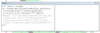
I then created a Multiple Ring Buffer around my interstates to see if the highest diesel concentrations were within this area and whether it had a proximity of 0 to 5 miles within the interstate or 5 to 10 miles within the interstate.  I did this by using a python script (Figure 1).

Figure 1. Python script used to create Multiple Ring Buffer for interstates.

I used a total distance of 10 miles because although diesel particulate matter of 2.5 in size can travel hundreds of miles, it seemed more reasonable to use a distance that seemed fairly close to the source that I hypothesized the diesel PM was coming from (pima.gov).

By adding a layer that contained diesel PM concentrations and using the 'Intersect' tool, I intersected the layer of diesel PM with my clipped buffered interstates to create the layer 'Diesel_interstates_intersect'.

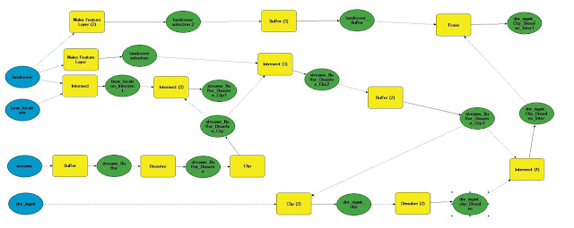
Lastly, I added a layer containing asthma emergency department visit rates within counties in California.  I intersected this data with the diesel PM/interstate buffer that I intersected previously.  This would allow me to see if higher asthma rates were within the 10 miles and the concentrated areas of Diesel PM.  The steps I followed throughout the process of analyzing my spatial question can be seen in the data flow model below (Figure 2).  Finalizing my methods, I created a cartographically pleasing map to show the results of my research.

Figure 2. Data flow model of the steps I took to accomplish my final project.

Results

My project resulted in some interesting data yet more research probably needs to be done to fully understand such a complex topic.  I found that most areas with a high concentration of diesel PM follow a similar pattern to that of the interstates.  These areas are also within the 10 miles road buffer I made and those with the largest concentrations appear to be within the closest road buffer having a proximity of 5 miles to an interstate.  When looking at the asthma data in comparison to concentrations, it appears to be less conclusive.  This may be because these values are taken from counties and each of these counties do not fully lie within the Central Valley.  However, some of the highest rates of asthma emergency department visits correlate with the areas of high diesel PM concentrations – based on towns with high diesel PM concentrations within these counties.  I plotted the towns that were within the 90 to 100 percentile diesel PM scores to show that they were within counties with the highest rates of asthma emergency department visits.

Figure 3. Locator map for the Central Valley of California.

Figure 4. Concentrations of diesel PM that are within 10 miles of interstates within the Central Valley.

Figure 5. Rates of asthma emergency department visits within the 10 mile buffer of interstates in the Central Valley.

Sources

Esri2017 Database (2017). [downloaded file (Asthma ED Visit Rates by County 2012)]. SQL Server. URL: geogsql.uwec.edu [May 11, 2017].

Esri2014 Database (2014). [downloaded file (CalEnviroScreen 2.0 Diesel PM Score)]. SQL Server. URL: geogsql.uwec.edu [May 11, 2017].

Esri2010 Database (2010). [downloaded file (Hypsographic map of California)]. SQL Server. URL: geogsql.uwec.edu [May 11, 2017].

What is Particulate Matter? (n.d.). Retrieved May 11, 2017, from http://dylosproducts.com/whispama.html

What is Particulate Matter? (n.d.). Retrieved May 11, 2017, from http://webcms.pima.gov/

GIS 1 Lab 5

Goals and Background:

In order to complete Lab 5, I needed a well-structured background on map overlay and geoprocessing to perform the correct relationships between layers.  To attain the knowledge I would need to accomplish this, my professor established interactive examples that examined functions/tools such as clip, erase, dissolve, intersect, and union.  I also completed tutorials that emphasized these points as well as walked me through the processes in making dataflow models.  The goal of Lab 5 was to demonstrate my understanding of geoprocessing tools and dataflow models to examine suitable bear habitats in Marquette County, Michigan and explore the basics of python scripting by analyzing the development of tourist resorts in Wisconsin and air pollution zones near interstates in Wisconsin.  As a result of completing this lab, a map of Marquette County, MI and two maps of Wisconsin displaying their respective goals along with dataflow models of each part of the lab will highlight my awareness of geoprocessing tools in ArcGIS.
Methods:
I began this lab by unzipping the supplied files and exploring each file type and coordinate system.  Moving on, I found I was given minimal data for bear_locations.  In order to determine the relationship between this feature class and the land cover type, I used the 'intersect' tool to develop a new feature class called 'bear_cover' that gave me the land cover information I needed to proceed.  With new criteria given to me pertaining to river resources for bears, I used a 'buffer' tool to create a distance of 500 meters surrounding a stream.  To clean this data up, I also performed the use of the 'dissolve' and 'clip' tools.  Once I selected the appropriate land covers (Mixed Forest Land, Forested Wetlands, and Evergreen Forest Land), I used the 'intersect' tool to intersect appropriate land covers and distances within rivers to find the ultimate suitable bear habitat.
I was then given more criteria disclosing DNR management lands and that these restoration areas should exclude areas within 5 kilometers of Urban or Built-up lands.  Therefore, I performed clipping and dissolving on DNR management lands to analyze those within the area of study.  I also performed a buffer and used the 'erase' tool to exclude within the areas mentioned previously.  Each tool used within this part of the lab can be found in the data flow model below (Figure 1).





Figure 1. Data flow model for criteria pertaining to suitable bear habitats and DNR management areas.

In part two of the lab I performed the python scripts shown below and developed more data models that explain each tool I used in the process of developing my final maps/analysis. Figure 2 through 5 illustrate lake resorts in WI (Section 1) and figures 6 and 7 display air pollution impact zones in WI (Section 2).


Figure 2. Python script for 10 mile buffer of cities in Wisconsin.

Figure 3. Python script for lakes with an area greater than 5 square miles.

Figure 4. Python script for clipping lakes that met criteria and buffered cities.

Figure 5. Dataflow model to develop suitable areas for the development of tourist resorts in Wisconsin.

Figure 6. Python script for making a multiple ring buffer around interstates in Wisconsin.

Figure 7. Dataflow modeling air pollution impact zones around interstates in Wisconsin.

Results:
Using the methods I performed above, I created three maps: one of suitable bear habitats in Marquette County in Michigan, one of possible lake resorts in Wisconsin, and one of air pollution hazards near interstates in Wisconsin.  Each of these maps are shown below.

Figure 8. Map of suitable bear habitats in Marquette County, Michigan.

Figure 9. Map of suitable lake areas for the development of tourist resorts.

Figure 10. Map of air pollution impact zones near Wisconsin interstates.

Sources:

Esri2017 Database (2017) [downloaded file]. SQL Server. URL: geogsql.uwec.edu [May 2, 2017]

Michigan Department of Natural Resources (2017) [downloaded file]. SQL Server. URL: geogsql.uwec.edu [May 2, 2017]


Price, Maribeth. 2016. Mastering ArcGIS. 7th Edition data. McGraw Hill. [downloaded file]. SQL Server. URL: geogsql.uwec.edu [May 2, 2017]


Wilson, Cyril 2012, A comprehensive Lake features for Wisconsin, Unpublished data. [downloaded file]. SQL Server. URL: geogsql.uwec.edu [May 2, 2017]